加速结构
光线追踪算法,开销大部分都在计算光线和三角形的交点上面,优化这个过程是必须的。加速结构的基础是BVH,这个就不详细解释了,不知道的可以自行了解。但实际的构建中,只有简单的BVH是不够的,这里我仿照目前现代引擎常用的BLAS/TLAS思想,构建整个场景的加速结构
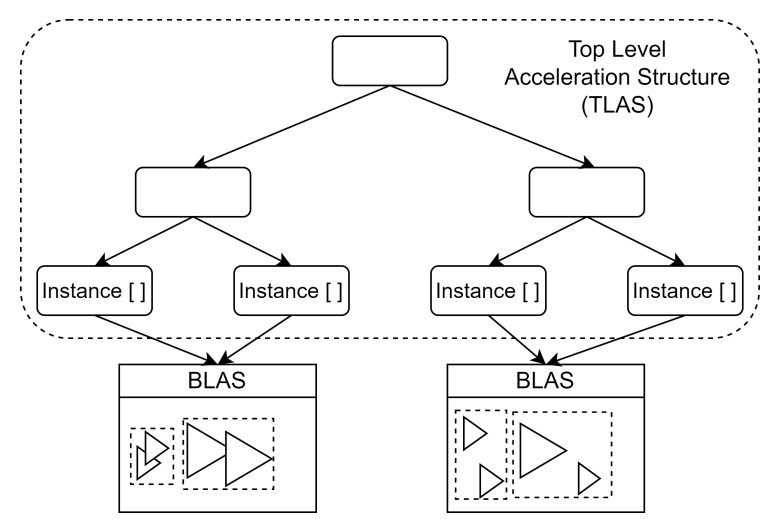
BLAS/TLAS
BLAS(Bottom-Level Acceleration Structure):
每个 BLAS 代表一个独立的几何体(如一个网格 Mesh)。
仅加速射线与该物体几何的相交测试。
通常内部是三角形的 BVH。
TLAS(Top-Level Acceleration Structure):
TLAS 管理的是多个 BLAS 的实例。
它保存每个实例的变换矩阵和世界空间的包围盒。
射线首先与 TLAS 相交,再变换到局部空间去查询 BLAS。
这种层级结构避免了重复构建和上传相同几何体的 BVH,只需变换即可复用。和上一章的object层级是一样的,之前每个Mesh都对应其变换矩阵和材质id,而一个Mesh实际上可以对应不同的变换矩阵,就创建了不同的实例
算法实现
具体实现时,很多地方都可以有多种方式,我这里给出一种折中且拓展性还不错的一种方案(./src/Scene.h):
// 轴对齐包围盒
struct alignas(16) AABB {
    alignas(16) glm::vec3 min = glm::vec3(FLT_MAX);
    alignas(16) glm::vec3 max = glm::vec3(-FLT_MAX);

    void expand(const glm::vec3& point) {
        min = glm::min(min, point);
        max = glm::max(max, point);
    }

    void merge(const AABB& other) {
        min = glm::min(min, other.min);
        max = glm::max(max, other.max);
    }

    glm::vec3 center() const { return 0.5f * (min + max); }
};

// BLAS 节点结构(适合 GPU 上传)
struct alignas(16) BLASNode {
    AABB bounds;
    glm::ivec3 indices = glm::ivec3(-1, -1, -1);   // 叶子节点用,对应叶子包含的三角形(最多3个,可拓展),其起始索引(在原始数据中),为局部(本Mesh)
    int left = -1;       // 内部节点索引
    int right = -1;      // 内部节点索引
};

class BLASBuilder {
public:
    struct Triangle {
        glm::vec3 v0, v1, v2;
        int index;  // 索引起始位置
    };

    struct BLAS {
        std::vector<BLASNode> nodes;
        std::vector<Triangle> triangles;
    };

    static BLAS buildBLAS(const Mesh* mesh);

private:
    static int buildRecursive(BLAS& blas, std::vector<Triangle>& tris, int begin, int end, std::vector<BLASNode>& nodes);

    inline static int maxAxis(const glm::vec3& v) {
        if (v.x > v.y && v.x > v.z) return 0;
        if (v.y > v.z) return 1;
        return 2;
    }
};

struct objectInfo{
    glm::mat4 transform;
    int materialID;
};

struct alignas(16) TLASInstance {
    glm::mat4 transform;
    AABB worldBounds;
    int rootNodeIndex; // 对应BLAS根节点位置
    int baseIndexOffset;
    int materialID;
    float padding;
};

class TLASBuilder {
public:
    struct alignas(16) TLASNode {
        AABB bounds;
        int left = -1;
        int right = -1;
        int instanceIndex = -1;  // 若为叶子节点
    };

    struct TLAS {
        std::vector<TLASInstance> instances;
        std::vector<TLASNode> nodes;
    };

    static TLAS buildTLAS(const std::vector<objectInfo>& objects, const std::vector<BLASBuilder::BLAS>& blasList);

private:
    static int buildRecursive(TLAS& tlas, int begin, int end, std::vector<TLASNode>& nodes);

    inline static int maxAxis(const glm::vec3& v) {
        if (v.x > v.y && v.x > v.z) return 0;
        if (v.y > v.z) return 1;
        return 2;
    }
};
直接从具体构建场景的加速结构的流程,来讲解上面的算法:
首先,为每个Mesh构建一个BLASBuilder::BLAS结构体,这里就是一个普通的BVH树,每个节点为BLASNode,当其为叶子时,这里为了设计方便,选择直接用一个向量存储该叶子包含的所有三角形的起始索引,所以构建时限制每个叶子最多三个三角形,这个后期也可以扩展
现在构建了所有Mesh的BLASBuilder::BLAS,形成了std::vector<BLASBuilder::BLAS>& blasList,上传至gpu时,会按顺序排列其中所有的BLASNode,所以在TLASInstance里,需要存储int rootNodeIndex;,对应了该Mesh的BVH树的根节点,这样从该根节点进入查询,就可以遍历其三角形。TLASInstance中还有int baseIndexOffset;,这是因为vertex和index也是按顺序堆叠的,而BLASNode中记录的三角形index为局部(本Mesh),所以需要记录每个Mesh的index偏移
然后调用TLASBuilder::buildTLAS(),传入所有的BLAS,构建场景的TLAS树,树的节点为TLASBuilder::TLASNode,当其为叶子时,通过instanceIndex来查询对应的实例,即TLASInstance,其中包含了实例的变换矩阵、材质id,以及BLAS的相关索引
具体怎么构建树,这里就不提了,都是最简单的BVH树构建方法,算法本身还有很多优化空间。两个树的根节点都会在最后面,这个可以通过调整递归位置来放在最前面,看个人选择
构建场景加速结构
继续从上一节的设计中派生方法class BLASBufferManager : public TypedBufferManager<BLASNode>;:
void collect(const std::vector<std::unique_ptr<Mesh>>& input) {
    meshes.clear();
    blasList.clear();
    obInfos.clear();
    meshes.reserve(input.size());
    for (const auto& m : input) {
        objectInfo info;
        info.transform = m->get_ModelMatrix();
        info.materialID = m->get_materialID();

        obInfos.push_back(info);
        meshes.push_back(m.get());
        blasList.push_back(BLASBuilder::buildBLAS(m.get()));
    }
}
首先收集场景的所有网格,记录每个网格的相关信息到std::vector<objectInfo> obInfos;,为每个网格生成BLAS结构
std::vector<BLASNode> fetch() const override {
    std::vector<BLASNode> result;
    uint32_t offset = 0;
    for (const auto& blas : blasList)
    {
        for (const BLASNode& n : blas.nodes)
        {
            BLASNode copy = n;                 // 做一份拷贝再改
            if (copy.left  >= 0) copy.left  += offset;
            if (copy.right >= 0) copy.right += offset;
            result.push_back(copy);
        }
        offset += static_cast<uint32_t>(blas.nodes.size());
    }
    return result;
}
接着要将信息调整为上传GPU的形式,即拼接所有的BLASNode,在拼接时,加上偏移,调整节点的左右指针为全局
TLASBufferManager类似,拿到上面创建好的信息后,构建TLAS结构,这里TLASInstance中两个全局偏移相关变量rootNodeIndex和baseIndexOffset很关键,在TLASBuilder::buildTLAS()中写入
着色器
在着色器中添加相关数据结构:
// binding = 2: BLASNode
struct AABB {
    vec3 min;
    vec3 max;
};
struct BLASNode {
    AABB bounds;
    ivec3 indices;
    int left;
    int right;
};
layout(std430, binding = 2) readonly buffer BLASBuffer {
    BLASNode blasNodes[];
};

// binding = 3: TLASInstance
struct TLASInstance {
    mat4 transform;
    AABB worldBounds;
    int rootNodeIndex; // 对应BLAS根节点位置
    int baseIndexOffset;
    int materialID;
};
layout(std430, binding = 3) readonly buffer TLASInstanceBuffer {
    TLASInstance instances[];
};

// binding = 4: TLASNode
struct TLASNode {
    AABB bounds;
    int left;
    int right;
    int instanceIndex;
};
layout(std430, binding = 4) readonly buffer TLASNodeBuffer {
    TLASNode tlasNodes[];
};
求交算法:
// 从 TLAS 开始进行包围盒遍历,并在叶子节点中调用 BLAS 进一步追踪
void traceTLAS_stack(int rootIndex, vec3 rayOrig, vec3 rayDir, inout float minT, inout vec3 hitColor) {
    int stack[MAX_STACK_SIZE];  // 遍历用的栈
    int sp = 0;                 // 栈指针
    stack[sp++] = rootIndex;   // 初始推入根节点

    while (sp > 0) {
        int nodeIndex = stack[--sp];              // 弹出当前节点索引
        TLASNode node = tlasNodes[nodeIndex];     // 获取当前 TLAS 节点

        // 如果射线未与该节点的 AABB 相交,跳过
        if (!intersectAABB(rayOrig, rayDir, node.bounds)) continue;

        // 叶子节点,表示是一个具体的实例
        if (node.left == -1 && node.right == -1) {
            int instanceIndex = node.instanceIndex;
            TLASInstance inst = instances[instanceIndex];  // 取出对应的实例信息
            mat4 model = inst.transform;                   // 实例的变换矩阵(局部 -> 世界)
            mat4 invModel = inverse(model);                // 世界 -> 局部(仅 BLAS 中使用)

            // 追踪该实例下的 BLAS
            traceBLAS_stack(inst.rootNodeIndex, rayOrig, rayDir, model, inst.materialID, inst.baseIndexOffset, minT, hitColor);
        } else {
            // 非叶子节点,将左右子节点入栈
            if (node.right >= 0) stack[sp++] = node.right;
            if (node.left >= 0)  stack[sp++] = node.left;
        }

        // 防止栈溢出
        if (sp >= MAX_STACK_SIZE) break;
    }
}
// 对一个具体的 BLAS 实例执行射线遍历和相交测试
void traceBLAS_stack(int rootIndex, vec3 rayOrig, vec3 rayDir, mat4 model, int materialID, int baseIndexOffset, inout float minT, inout vec3 hitColor) {
    int stack[MAX_STACK_SIZE];
    int sp = 0;
    stack[sp++] = rootIndex;

    // 把射线从世界空间变换到局部空间(与网格对齐)
    mat4 invModel = inverse(model);
    vec3 localOrigin = vec3(invModel * vec4(rayOrig, 1.0));
    vec3 localDir = normalize(mat3(invModel) * rayDir);

    while (sp > 0) {
        int nodeIndex = stack[--sp];
        BLASNode node = blasNodes[nodeIndex];

        // 局部空间下与 AABB 不相交,跳过
        if (!intersectAABB(localOrigin, localDir, node.bounds)) continue;

        // 叶子节点:执行三角形相交测试
        if (node.right < 0 && node.left < 0) {
            for (int i = 0; i < 3; ++i) {
                int localIndex = node.indices[i];
                if (localIndex == -1) break; // 无效索引跳过

                int idx = baseIndexOffset + localIndex;

                // 取出三角形顶点(局部空间)
                vec3 v0 = vertices[indices[idx + 0]].Position;
                vec3 v1 = vertices[indices[idx + 1]].Position;
                vec3 v2 = vertices[indices[idx + 2]].Position;

                float t;
                // 射线与三角形求交,t 为局部空间下的距离
                if (intersectTriangle(localOrigin, localDir, v0, v1, v2, t)) {
                    // 命中点从局部转到世界空间
                    vec3 hitLocal = localOrigin + t * localDir;
                    vec3 hitWorld = vec3(model * vec4(hitLocal, 1.0));
                    float tWorld = length(hitWorld - rayOrig); // 世界空间距离

                    // 如果距离更小,更新最小距离和命中颜色
                    if (tWorld < minT) {
                        minT = tWorld;
                        hitColor = materials[materialID].baseColor;
                    }
                }
            }
        } else {
            // 非叶子节点,压入左右子节点
            if (node.right >= 0) stack[sp++] = node.right;
            if (node.left >= 0)  stack[sp++] = node.left;
        }

        if (sp >= MAX_STACK_SIZE) break;
    }
}
注释的应该比较明白了,整体就是一个栈实现的深度搜索,思路如下:
traceTLAS_stack()
└── 遍历 TLAS(世界空间)
    └── 命中某个 TLAS 叶子 → 获取 instance 数据
        └── traceBLAS_stack()
            └── 在该实例中进行 BLAS 局部空间遍历 + 三角形求交
                └── 若命中:反变换得到世界空间交点 → 更新 minT 和 hitColor
在主循环中,只需要:
// 2. 初始化 hit 信息
float minT = 1e20;
vec3 hitColor = vec3(0.0);

// 3. 遍历 TLAS 根节点(最后一个)
int tlasRoot = int(tlasNodes.length()) - 1;
traceTLAS_stack(tlasRoot, rayOrig, rayDir, minT, hitColor);
就可以拿到交点颜色,后续也很简单的可以扩展为获取交点的法线、纹理坐标等,这里先保持简单一点
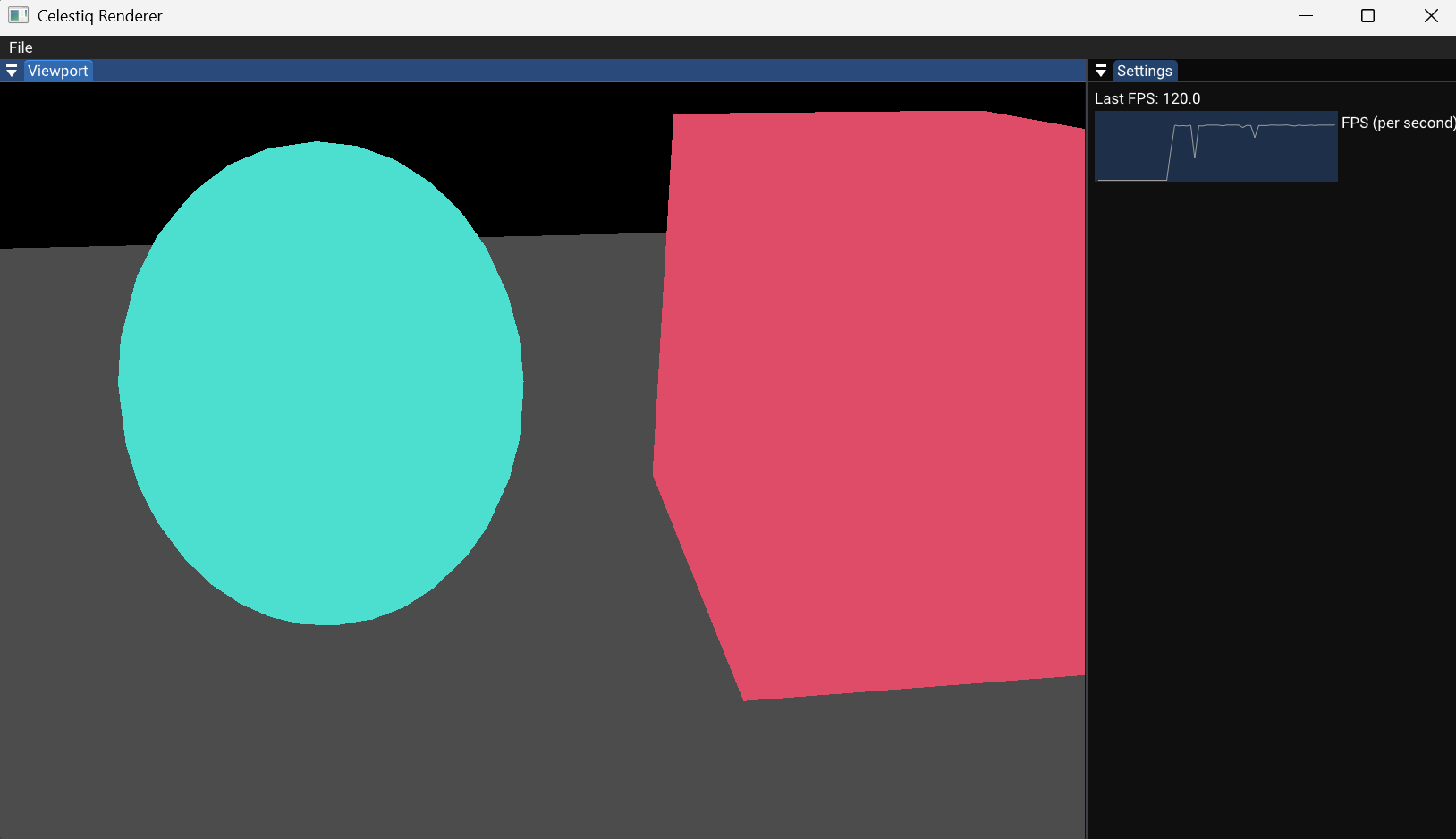
构建
添加了一个显示帧率的ui,可以看到,基本上顶满了上限120帧在跑(取决于显示器),比上一节直接遍历场景高了一倍左右。这里只有一千左右个面,当场景变得更加复杂时,提升会更加明显
代码存档
代码下载